The index match formula is one of Excel’s most powerful and flexible lookup functions that every data analyst should master.
While many Excel users rely on VLOOKUP for data retrieval, the index match formula offers superior flexibility and performance that can transform how you handle complex data analysis tasks.
Table of Contents
What Makes INDEX MATCH Superior to Other Lookup Functions?
When working with large datasets, the index match formula stands out as a game-changer.
VLOOKUP can only look for values to the right of your lookup column, whereas INDEX and MATCH let you search in either direction.
This versatility makes it an essential tool for anyone serious about Excel proficiency.
The index match formula combines two separate Excel functions: INDEX and MATCH.
With INDEX, you can pull out the actual value stored at a certain spot in a range, whereas MATCH tells you the relative position of a value within that range.
Together, they create a dynamic duo that outperforms traditional lookup methods in both speed and functionality.
Many Excel professionals consider the index match formula their go-to solution because it doesn’t break when columns are inserted or deleted.
This reliability factor alone makes it worth learning, especially when working with evolving spreadsheets that require consistent data retrieval.
Understanding the Basic Syntax
The index match formula follows a straightforward structure that becomes intuitive with practice. The basic syntax combines INDEX and MATCH functions in a nested format:
excel
=INDEX(return_array, MATCH(lookup_value, lookup_array, 0))Let’s break down each component of this index match formula:
- return_array: The column or range that contains the values you need to return.
- lookup_value: The value you’re searching for.
- lookup_array: The column or range where the values you want to look up are located.
- 0: This option specifies an exact match — always set it to 0 if you want precise results.
This structure makes the index match formula incredibly flexible. You can look up data in any column and pull values from another column, no matter where they are located in the worksheet.
Step-by-Step Implementation Guide
Getting started with the index match formula requires understanding the logical flow of the function. First, identify what value you need to find (your lookup value) and where it’s located.
Then, determine which column contains the information you want to retrieve.
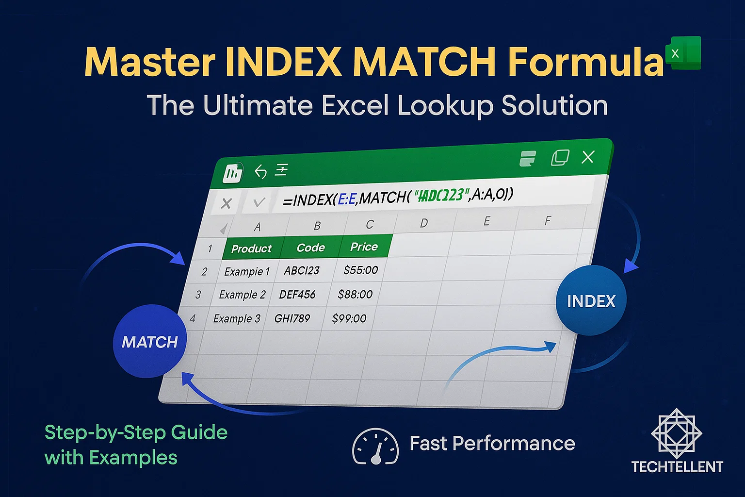
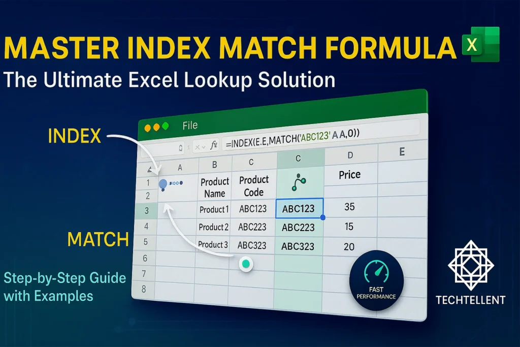
Consider a practical example: you have a product database with item codes in column A and prices in column E.
To find the price for item “ABC123”, your index match formula would look like this:
excel
=INDEX(E:E, MATCH("ABC123", A:A, 0))This index match formula tells Excel to find “ABC123” in column A, determine its row position, and return the corresponding value from column E.
The beauty of this approach is that it works regardless of how many columns exist between your lookup and return columns.
For more complex scenarios, you might need to reference cells instead of hard-coding values. A dynamic index match formula using cell references would be:
excel
=INDEX($E:$E, MATCH(B2, $A:$A, 0))The dollar signs create absolute references for the arrays while allowing the lookup value (B2) to change when you copy the formula to other cells.
Advanced INDEX MATCH Techniques
Once you’ve mastered the basic formula, you can explore more sophisticated applications. Two-way lookups represent one of the most powerful uses of this function combination.
A two-way lookup uses the index match formula to search both horizontally and vertically.
This technique is perfect for matrix-style data where you need to find values at the intersection of specific rows and columns:
excel
=INDEX(data_range, MATCH(row_lookup, row_headers, 0), MATCH(column_lookup, column_headers, 0))This advanced index match formula structure allows you to create dynamic reports that adapt to changing criteria.
Sales managers often use this technique to quickly locate specific product performance data across different time periods or regions.
Another powerful application involves using the formula with multiple criteria. Although older versions of Excel need array formulas for this, it highlights how flexible the function is:
excel
=INDEX(return_array, MATCH(1, (criteria1_range=criteria1)*(criteria2_range=criteria2), 0))Performance Comparison: INDEX MATCH vs Other Functions
The index match formula consistently outperforms other lookup functions in both speed and reliability tests. Here’s a comparison of common lookup methods:
| Function | Speed | Flexibility | Column Limitation | Memory Usage |
|---|---|---|---|---|
| INDEX MATCH | Fast | Very High | None | Low |
| VLOOKUP | Medium | Limited | Right side only | Medium |
| XLOOKUP | Fast | High | None | Medium |
| HLOOKUP | Medium | Limited | Below only | Medium |
| FILTER | Slow | High | None | High |

This comparison clearly shows why experienced Excel users prefer the index match formula for most lookup scenarios. The combination of speed, flexibility, and low memory usage makes it ideal for large datasets and complex workbooks.
The index match formula also handles errors more gracefully than VLOOKUP. When a lookup value isn’t found, you can easily wrap the formula in IFERROR to provide meaningful feedback:
excel
=IFERROR(INDEX(return_array, MATCH(lookup_value, lookup_array, 0)), "Not Found")Common Mistakes and Troubleshooting
Even experienced users sometimes encounter issues with the index match formula. The most common problem involves mismatched data types between lookup values and the lookup array.
Excel requires exact matches, so text formatted as numbers won’t match actual numbers.
Another frequent issue occurs when the index match formula returns unexpected results due to duplicate values in the lookup array.
The MATCH function always returns the first occurrence, which might not be the desired result in datasets with repeated entries.
To avoid these problems, always verify your data types and consider using helper columns to concatenate multiple criteria when dealing with potential duplicates.
The index match formula works best with clean, well-structured data.
Circular references represent another pitfall when building complex models with the index match formula.
Always ensure your lookup arrays don’t include the cells where you’re placing your formulas.
Real-World Applications and Examples
The index match formula shines in practical business scenarios. Human resources departments use it to quickly retrieve employee information from comprehensive databases.
By entering an employee ID, HR staff can instantly access salary information, department details, or performance metrics.
Financial analysts rely on the index match formula for building dynamic financial models.
When creating budget reports that need to pull data from multiple worksheets, this function combination provides the reliability and speed necessary for professional-grade analysis.
Inventory management represents another excellent use case for the index match formula.
Warehouse managers can create lookup systems that instantly display stock levels, supplier information, and reorder points by simply entering product codes.
For those looking to expand their Excel skills further, www.techtellent.com offers comprehensive tutorials on advanced Excel functions and data analysis techniques.
Integration with Other Excel Functions
The true power of the index match formula emerges when combined with other Excel functions.
Creating dynamic ranges with OFFSET and the index match formula allows for incredibly flexible reporting systems that automatically adjust to growing datasets.
Statistical functions like SUMPRODUCT work beautifully with the index match formula to create conditional aggregations.
This combination enables complex business intelligence reports that would be difficult or impossible with traditional lookup functions.
Microsoft’s official Excel documentation provides extensive examples of these advanced combinations, demonstrating why the index match formula remains a cornerstone of professional Excel use.
Related Excel Resources and Advanced Learning
Now that you’ve mastered the index match formula, you can apply this knowledge to various Excel projects and templates.
Understanding lookup functions becomes especially valuable when working with complex business scenarios and automated reporting systems.
If you’re just starting your Excel journey, our comprehensive Excel for Beginners PDF guide provides foundational knowledge that complements the index match formula techniques covered here.
This resource helps you build the groundwork necessary for advanced formula applications.
For project management applications, the index match formula works exceptionally well with structured templates like our Google Sheets Product Roadmap Template.
While designed for Google Sheets, the lookup principles transfer perfectly to Excel environments where you need dynamic data retrieval for project tracking.
Financial professionals will find the index match formula particularly useful when working with our specialized templates.
The Debt Service Coverage Ratio Formula in Excel guide demonstrates how lookup functions integrate with financial calculations.
Similarly, our Profit Margin Formula Excel Guide shows practical applications of the index match formula in financial analysis scenarios.
Business process optimization benefits greatly from the index match formula’s flexibility. Our RFI Template Excel guide showcases how lookup functions streamline vendor management and procurement processes.
The same principles apply to customer relationship management in our Real Estate CRM Excel Template, where the index match formula enables quick client information retrieval.
Reporting automation represents another powerful application area. Our Monthly Sales Report Template in Excel leverages lookup functions similar to the index match formula for dynamic report generation.
For debt management scenarios, the Debt Schedule Template Excel demonstrates how lookup functions create flexible payment tracking systems.
Advanced Excel users should explore our guide on how to Automate Excel Reports using best practices, which shows how the index match formula integrates with other automation techniques.
Additionally, our Pivot Table Practice Exercises complement lookup function skills by teaching another essential data analysis method.
These resources work together to create a comprehensive Excel skill set where the index match formula serves as a fundamental building block for more complex data manipulation and analysis tasks.
Conclusion
Mastering the index match formula transforms your Excel capabilities from basic to professional level.
This powerful function combination offers unmatched flexibility, superior performance, and reliable results that make it essential for serious data analysis.
Whether you’re managing inventory, analyzing sales data, or building complex financial models, the index match formula provides the robust lookup functionality you need.
Its ability to search in any direction, handle large datasets efficiently, and integrate seamlessly with other Excel functions makes it an indispensable tool.
Start incorporating the index match formula into your daily Excel work, and you’ll quickly discover why it’s considered the gold standard for lookup functions.
With practice, this versatile formula will become second nature, opening up new possibilities for data analysis and reporting that you never thought possible.