AVERAGEIFS is one of Excel’s most powerful statistical functions that allows users to calculate conditional averages based on multiple criteria.
This advanced AVERAGEIFS function serves as an essential tool for data analysts, business professionals, and anyone working with complex datasets who needs to extract meaningful insights from their spreadsheets.
Understanding how to use the AVERAGEIFS function effectively can transform your data analysis capabilities, making you more efficient and accurate in your calculations.
Whether you’re analyzing sales performance, student grades, or financial metrics, the AVERAGEIFS function provides the flexibility to average values while meeting specific conditions across multiple columns.
Table of Contents
🎯 What is the AVERAGEIFS Function?
The AVERAGEIFS function calculates the arithmetic mean of cells that meet multiple specified criteria.
Unlike its simpler counterpart, the AVERAGEIFS function excels at handling complex scenarios where you need to apply several conditions simultaneously to determine which values should be included in your average calculation.
This AVERAGEIFS statistical function follows a specific syntax that allows users to define multiple criteria ranges and their corresponding conditions.
The beauty of the AVERAGEIFS function lies in its ability to process multiple logical tests at once, making it incredibly useful for sophisticated data analysis tasks.
When working with large datasets containing thousands of rows, the AVERAGEIFS function becomes invaluable for filtering and calculating averages based on specific parameters.
This function eliminates the need for complex filtering operations or multiple helper columns that would otherwise clutter your worksheet.

📝 Understanding the AVERAGEIFS Syntax Structure
The syntax structure for the AVERAGEIFS function follows a logical pattern that makes it relatively straightforward to implement once you understand the components:
=AVERAGEIFS(average_range, criteria_range1, criteria1, [criteria_range2, criteria2], ...)Let’s break down each component:
- average_range: The range of cells you want to calculate the average for
- criteria_range1: The first range to evaluate against your first criterion
- criteria1: The condition that must be met in criteria_range1
- criteria_range2, criteria2: Additional optional criteria ranges and conditions
This flexible syntax allows you to include up to 127 criteria pairs, making the AVERAGEIFS function incredibly powerful for complex analytical tasks.
The AVERAGEIFS function evaluates all conditions using AND logic, meaning all criteria must be satisfied for a cell to be included in the average calculation.
🔍 How AVERAGEIFS Differs from Other Excel Functions
When comparing the AVERAGEIFS function with other Excel averaging functions, several key distinctions emerge.
The standard AVERAGE function simply calculates the mean of a range without any conditions, making it suitable for basic calculations but limited for analytical work.
The AVERAGEIF function allows for single-criterion averaging, which works well for simple conditional calculations.
However, AVERAGEIFS surpasses both by enabling multiple criteria evaluation, making the AVERAGEIFS function the go-to choice for complex data analysis scenarios.
Unlike AVERAGEA, which includes text and logical values in its calculations, the AVERAGEIFS function focuses purely on numerical data that meets your specified conditions.
This focused approach ensures more accurate results when working with mixed data types.
For more advanced Excel techniques and functions, visit TECH TELLENT for comprehensive tutorials and guides that can enhance your spreadsheet skills.
💡 Practical Examples in Action
Let’s explore several real-world scenarios where this conditional averaging function proves invaluable. Consider a sales dataset where you need to calculate average sales amounts for specific regions and time periods simultaneously.
=AVERAGEIFS(D2:D100, B2:B100, "North", C2:C100, ">1000")This formula calculates the average of values in column D where column B contains “North” and column C contains values greater than 1000.
Such calculations would require multiple steps with simpler functions but are accomplished effortlessly with this powerful Excel tool.
Another common application involves analyzing student performance data. You might want to calculate the average score for students in a specific grade level who scored above a certain threshold:
=AVERAGEIFS(E2:E200, C2:C200, "Grade 10", E2:E200, ">=75")This example demonstrates how this function can reference the same range in both the average_range and criteria_range parameters, providing flexibility in your analysis approach.
📊 Sample Data Analysis with Multiple Criteria
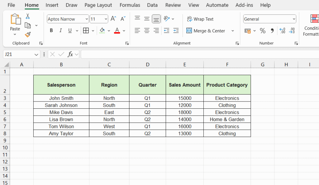
Here’s a comprehensive example using a sales performance dataset:
| Salesperson | Region | Quarter | Sales Amount | Product Category |
|---|---|---|---|---|
| John Smith | North | Q1 | 15000 | Electronics |
| Sarah Johnson | South | Q1 | 12000 | Clothing |
| Mike Davis | East | Q2 | 18000 | Electronics |
| Lisa Brown | North | Q2 | 14000 | Home & Garden |
| Tom Wilson | West | Q1 | 16000 | Electronics |
| Amy Taylor | South | Q2 | 13000 | Clothing |

Using this data, you can create various conditional averaging formulas:
=AVERAGEIFS(D2:D7, B2:B7, "North", E2:E7, "Electronics")This formula would calculate the average sales amount for the North region in the Electronics category, demonstrating how this Excel function handles multiple criteria across different columns.
🚀 Advanced Tips for Effective Usage
Mastering this conditional averaging tool requires understanding several advanced techniques that can significantly improve your analytical capabilities.
When working with date ranges, you can use comparison operators to create dynamic time-based criteria:
=AVERAGEIFS(A2:A100, B2:B100, ">=1/1/2023", B2:B100, "<=12/31/2023")This approach allows you to calculate averages for specific date ranges without manually filtering your data.
The function automatically evaluates date criteria and includes only the relevant records in its calculation.
Wildcard characters add another layer of flexibility to your conditional averaging formulas.
Using asterisks (*) and question marks (?), you can create partial text matches that expand your filtering capabilities:
=AVERAGEIFS(C2:C50, A2:A50, "Sales*", B2:B50, ">500")This formula averages values where column A starts with “Sales” and column B is greater than 500, demonstrating how wildcards enhance your criteria flexibility.
⚠️ Common Mistakes to Avoid
Several pitfalls can compromise your results if not addressed properly. Range size mismatches represent the most frequent error, where your average_range and criteria_range parameters contain different numbers of cells.
Ensure all ranges have identical dimensions to prevent calculation errors. Excel may not always generate error messages for size mismatches, potentially leading to incorrect results that could impact your analysis.
Text formatting issues can also cause problems with these calculations.
Extra spaces, inconsistent capitalization, or hidden characters in your criteria cells can prevent the function from finding matches.
Consider using TRIM and UPPER functions to clean your data before applying conditional averaging.
Data type conflicts occur when your criteria reference cells containing different data types than expected.
For instance, comparing text criteria against numerical ranges or vice versa can yield unexpected results.
🛠️ Troubleshooting Function Issues
When your conditional averaging formulas return unexpected results, systematic troubleshooting can identify and resolve the underlying problems.
Start by verifying that your criteria ranges and average range contain the expected data types and formats.
Use Excel’s formula evaluation tool to step through your calculations, observing how each criterion is processed.
This approach helps identify which specific conditions might be failing or producing unexpected matches.
Consider breaking complex formulas into smaller components to isolate problematic criteria.
Test each criterion individually using COUNTIFS to verify that your conditions are identifying the correct records before calculating averages.
Excel’s external documentation provides additional resources for resolving complex function issues.
Microsoft’s official Excel help documentation offers detailed explanations and troubleshooting guides for advanced functions like this conditional averaging tool.
📈 Optimizing Performance with Large Datasets
Large datasets can impact performance, especially when working with thousands of rows and multiple criteria.
Several optimization techniques can improve calculation speed and reduce processing time.
Minimize the size of your criteria ranges by using only the necessary cells rather than entire columns.
Instead of referencing A:A, use specific ranges like A2:A1000 to reduce Excel’s processing overhead.
Consider using structured references with Excel tables, which can improve both performance and formula readability.
Table references automatically adjust when you add or remove data, maintaining your formula accuracy without manual updates.
Array formulas and dynamic arrays in newer Excel versions can sometimes provide performance improvements over traditional implementations, particularly with complex multi-criteria scenarios.
🎓 Best Practices for Implementation
Successful implementation relies on following established best practices that ensure accuracy and maintainability.
Always document your criteria logic clearly, either through comments or separate documentation, so others can understand your analysis approach.
Use named ranges for frequently referenced data ranges, making your formulas more readable and easier to maintain.
Named ranges also reduce the likelihood of errors when copying formulas to different locations.
Implement data validation on your criteria inputs to prevent users from entering invalid values that could compromise your calculations.
This proactive approach maintains data integrity and ensures reliable results.
Regular testing of your conditional averaging formulas with known datasets helps verify that your calculations remain accurate as your data changes over time.
❓ Frequently Asked Questions About AVERAGEIFS
Can this function handle more than two criteria?
Yes, AVERAGEIFS can accommodate up to 127 criteria pairs, making it extremely flexible for complex analytical requirements. This means you can apply dozens of different conditions simultaneously to filter your data before calculating the average.What happens if no cells meet all the specified criteria?
The function returns a #DIV/0! error when no cells satisfy all conditions, indicating that no data points were found for averaging. This error helps you identify when your criteria might be too restrictive or when there’s no matching data.Can I use cell references for criteria in this function?
Absolutely. You can reference cells containing your criteria values, making your formulas dynamic and easier to modify. This approach allows you to change criteria without editing the formula itself.Does this function work with text criteria?
Yes, it supports both numerical and text criteria, including wildcard characters for partial matches. You can use asterisks (*) and question marks (?) to create flexible text-based conditions.How does this function handle blank cells in the average range?
The function ignores blank cells in the average range, focusing only on numerical values that meet your specified criteria. This ensures accurate calculations without interference from empty cells.Is there a limit to how many criteria I can use?
Excel allows up to 127 criteria pairs in a single formula. However, practical limitations may arise based on your worksheet size and system performance with extremely complex formulas.Can this function work with dates as criteria?
Yes, it handles date criteria effectively. You can use comparison operators like >=, <=, and = with dates to create time-based filtering conditions for your average calculations.🔚 Conclusion
AVERAGEIFS stands as one of Excel’s most versatile and powerful functions for conditional data analysis.
Its ability to process multiple criteria simultaneously makes it indispensable for professionals working with complex datasets requiring sophisticated filtering and calculation capabilities.
Mastering this conditional averaging function opens doors to advanced analytical possibilities that can significantly enhance your data processing efficiency.
From sales performance analysis to academic grade calculations, this tool provides the flexibility and precision needed for professional-quality spreadsheet work.
The investment in learning this powerful Excel function pays dividends through improved analytical capabilities, reduced processing time, and more accurate results.
As your data analysis requirements grow more complex, this multi-criteria averaging tool will prove increasingly valuable in your Excel toolkit.
Remember that practice makes perfect when working with advanced Excel functions.
Start with simple examples and gradually increase complexity as your confidence grows with this powerful analytical tool.
💬 Your Support Means Everything
Have you found this guide helpful in understanding this powerful Excel function?
We’d love to hear about your experiences using this conditional averaging tool! Share your success stories, creative applications, or any challenges you’ve encountered in the comments below.
Your insights help build a stronger community of Excel enthusiasts, and your unique perspective might be exactly what another reader needs to solve their data analysis puzzle.
Don’t hesitate to leave a comment – every contribution makes our learning community better!

marijuana gummies online with safe packaging